
Robotic Systems Laboratory
The goal of the Robotic Systems Laboratory project was to enable a mobile robot to autonomously navigate a maze using control mechanisms, mapping techniques, localization methods, and path planning algorithms. The robot is capable of mapping its surroundings, identifying its location, and traversing from the starting point to the destination using controlled motion signals.

Equipment
The robot utilized for this project is a differential drive type, outfitted with an IMU, a camera, 2D LiDAR, motors, a Raspberry Pi, and a Beaglebone Blue.

Control
We used a PID controller for the robot's velocity and motion. It adjusts speed and direction by reducing the difference between desired and actual values. The controller has three parts: Proportional (P) for immediate error, Integral (I) for accumulated errors, and Derivative (D) for anticipating errors. This ensures precise robot movement along the desired path.
To minimize noise levels, we implemented a 1st order Butterworth Low Pass Filter (LPF) on both the encoder velocity and the motor Pulse Width Modulation (PWM) command. The selection of the filter's order and its cutoff frequency was determined through a process of trial and error, guided by observations from the velocity plots. Additionally, a 1st Order LPF was applied to the input velocity setpoint. This filtering of the setpoint transformed the step input into a gradual, linear input over a brief period, diminishing the system's initial overshoot.

Mapping
We utilized the robot's LiDAR to generate a 2D occupancy map of its surroundings. An occupancy map represents a discretization of the state space into 2D grid cells, each holding a probability of being occupied or free. By interpreting the distances measured by the LiDAR rays, we can determine the probability of a cell being occupied (black) or free (white). With the robot's continuous movement and scanning, the status of the cells is updated using Bayes' Theorem.
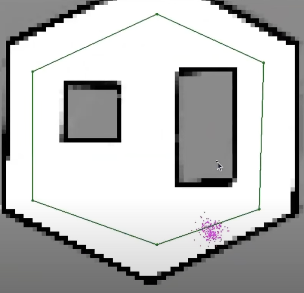
Localisation
In order for the robot to know its location with respect to its environment, we used particle filter localisation. A technique in which particles are distributed uniformly over the configuration space. Each particle represents a possible state where the robot could be. Through observations and movements in the environment, the algorithm resamples particles with Bayesian estimation in locations where the robot most likely will be. The process continuous until the large majority of particles converge to the actual location of the robot.
Path Planning
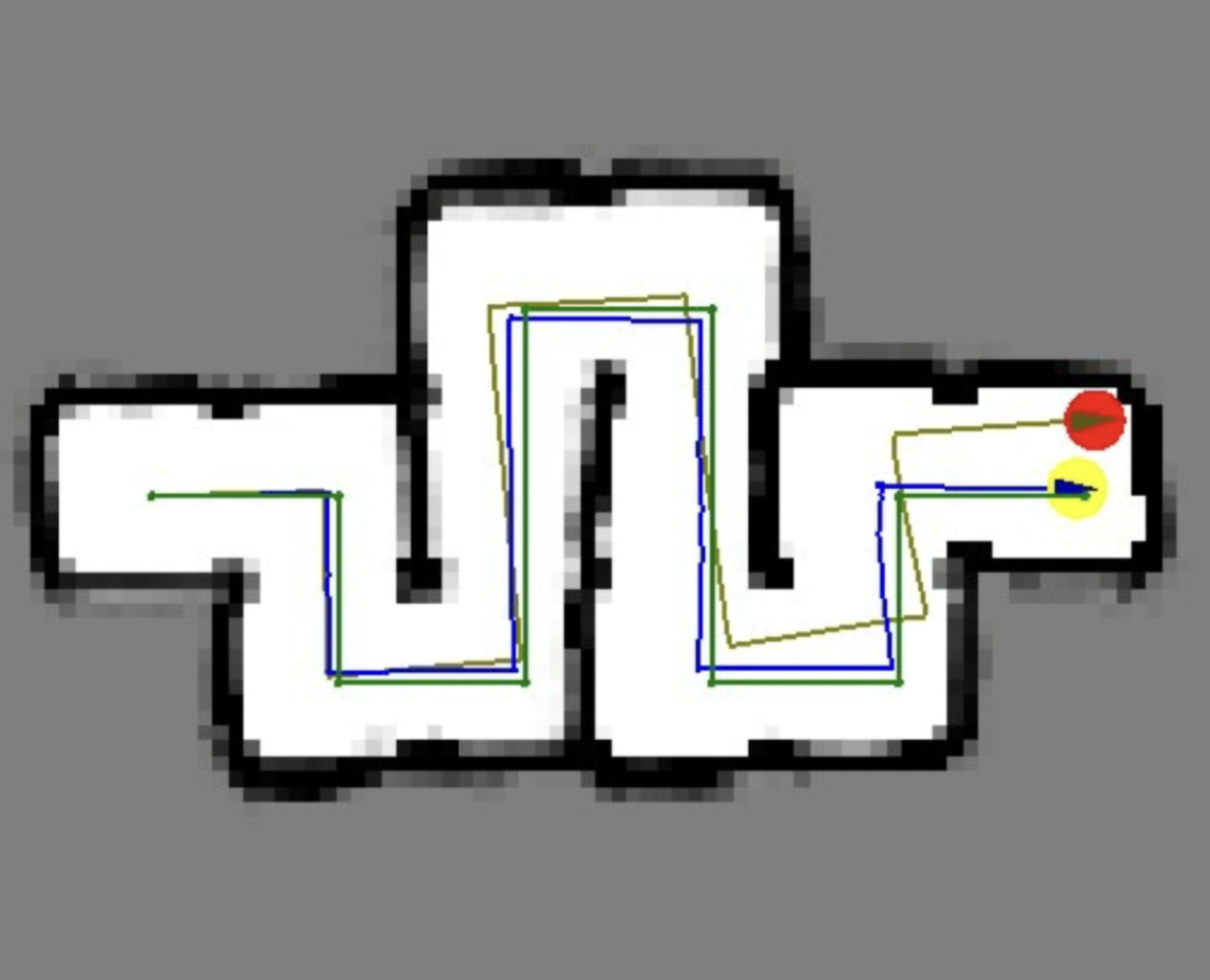
The robot employs the A* algorithm to plan a path from its initial position to its destination. It combines the actual distance traveled with a heuristic to estimate the remaining distance to the target, prioritizing the exploration of nodes with the lowest combined cost, thereby efficiently finding the optimal path.
Image: A* Path (green) overlayed with Robot Path(blue) on custom map (black cells).
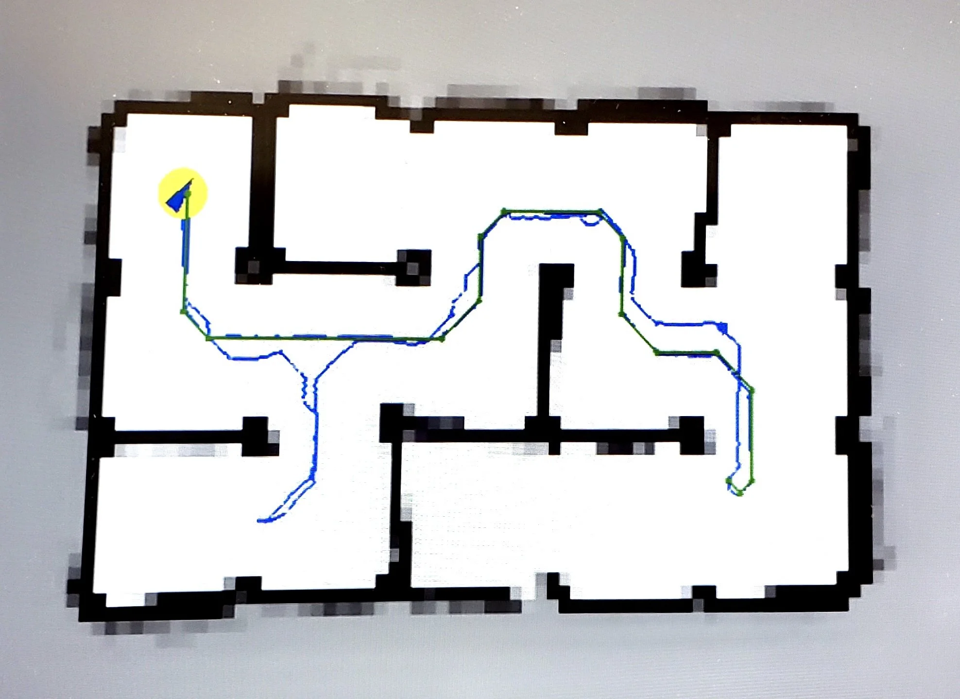
SLAM vs. Odometry
A map was generated from a maze that the robot traversed, following specified waypoints. Brown denotes the odometry readings, while blue signifies the SLAM pose. This differentiation underscores the importance of SLAM and sensor fusion in applications of mobile robotics.
Results
The video below showcases the robot navigating through the maze. It is capable of mapping its surroundings, identifying its location, and traversing from the starting point to the destination using controlled motion signals